Lead
Choosing a set of initial conditions that would be likely to produce a successful liquid chromatography (LC) separation was the main topic of discussion in the first post in the HPLC method development series. The majority of samples will benefit from starting with a C8 or C18 column packing based on Type B silica using a mobile phase of acetonitrile or methanol modified with water or a low-pH buffer, even though no single set of starting conditions will ensure success. During the next posts the focus was on the importance of being able to measure the characteristics of the separation quantitatively in order to address a similar issue with LC separations. Retention time (tR), retention factor (k), peak asymmetry or U.S. Pharmacopeia tailing factor (Tf), column plate number (N), and resolution (RS) were the specific measurements of interest.
In this and forthcoming post, we will see how these tools can be employed to guide chromatographers to achieve successful separation. The fundamental resolution equation (equation 1) in particular will make it easier to assess how different selectivity-controlling variables will affect a method’s performance. An overview of the variables that control chromatographic separation is depicted in the image below.
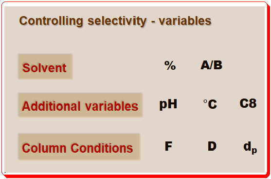
Note: details of abbreviations used is given below;
- Solvent: strength (% ), composition (A (aqueous)/B (organic)
- Additional variables: pH, Temperature (°C), Column packing (C8 or C18, etc.)
- Column conditions: Flow (F), Dimension , Particle size (dp)
Resolution is crucial
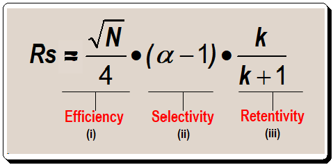
Separating one or more sample components from other components in a sample is the aim of the chromatographic process. Measurement of resolution was discussed in the last post [https://chiralpedia.com/blog/measuring-quality-of-chromatogram-tools-3-0/ ]. The valley between two peaks reaches the baseline at about a 1.5 resolution. The majority of workers prefer separations with resolution values greater than 1.7 because they allow for some separation loss without rendering the separation useless. Similar to this, most applications don’t benefit much when resolution exceeds 2.0; run times increase without any noticeable qualitative improvement. The basic resolution equation shown below is a helpful tool to direct the process of getting a good separation for method development purposes. The focus of this post will be on terms ii and iii in equation I.
Consider the connection between term iii of equation 1 and resolution before delving into the specifics of controlling selectivity. Let us plot the terms retention factor (k) in the X-axis and resolution (RS ) in the Y-axis , as in Figure 1, to understand the relationship between them.
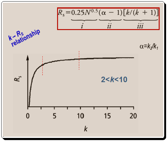
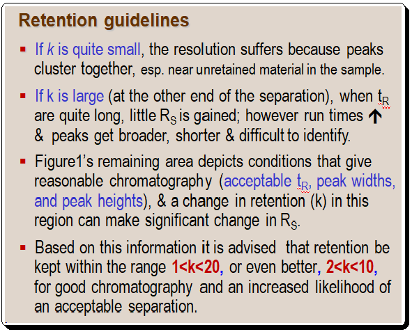
Finally, equations 1 and 2 ( α = k2/k1) demonstrate how peak spacing (α) also varies with retention. The general improvement in resolution that occurs as retention rises is caused by this relationship (Figure 1). (Remember that k in equation 1, part (iii) is equal to the average of k1 and k2 values equation 2). A retention guidelines is presented below:
Solvent role
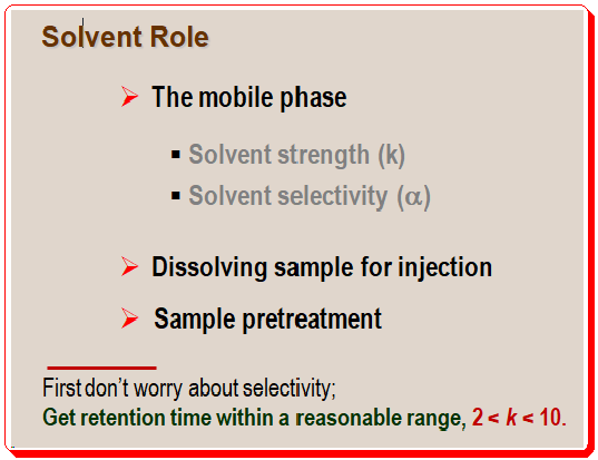
First Approach: Adjust solvent strength
Stepwise-exploration:
Prior to becoming overly concerned with selectivity, it’s critical to get the retention time within a manageable range. In an isocratic separation mode, one may go with a step-wise exploration approach by changing the strength of the organic solvent. Here, you may start with 90% or 100% solvent B (organic solvent) concentration and decrease the concentration by 10% steps to adjust retention. Run solvent B at 100%, 90%, 80%, and so forth until retention times are in the 1–20 range, which is ideal for good chromatographic behavior.
Figure 2 shows the first three runs in this series. According to equation 1 and Figure 1, the retention and resolution increase as the organic solvent concentration decreases from 80% to 70% to 60%. A 150 mm x 4.6 mm column running at a 1.5 mL/min flow rate was used for the runs in Figure 2, meaning t0 is approximately 1 minute. A quick review of the chromatogram for the 60% B mobile phase enables a very accurate estimation of the retention factor of 2 < k < 7. The separation doesn’t require much optimization because the peaks are baseline resolved and the run time is brief.
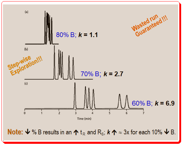
As the organic content of the mobile phase changes, you find that the peaks in Figure 2 are moving in a predictable pattern. The general peak movements is guided by the Rule of Three. According to this general rule, retention factors will roughly triple for every 10% decrease in the mobile phase’s organic-solvent content. The k values for the last peak in the runs of Figure 2 are 1.1, 2.7, and 6.9, so the Rule of Three is quite useful as a general rule of thumb, but for this specific sample, the Rule of 2.5 works better. Finally, keep in mind that the retention factor changes by threefold for every 10% change, so a 20% change in solvent B would result in a 3 x 3 or approximately 9 fold change.
Fine-tuning mobile phase composition:
Every peak in Figure 2 follows the pattern shown in Figure 1. That is, as the mobile-phase strength is decreased, retention and resolution rise. Despite being a generalization, this pattern of change fortunately does not apply to all compounds. The exceptions to the rule are significant because they give chromatographers the opportunity to adjust the mobile-phase composition and improve selectivity in separation.
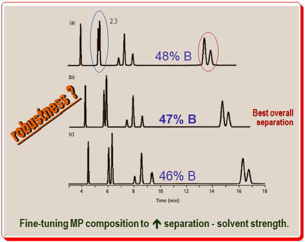
Figure 3 shows how you can enhance a separation by carefully tuning the mobile-phase composition. Similar to Figure 2, the mobile phase in Figure 3 becomes weaker from top to bottom (48 to 46% of organic solvent). Likewise, you can see that with a lower percentage of solvent B, peak 2 and peak 3 (marked in blue oval circle) resolution improves and simultaneous increase in the retention time. However, pay attention to how the final two peaks ( marked in red oval circle) in each run change over time. This peak pair’s resolution shifts in the opposite direction. The general pattern of longer retention and better resolution with weaker mobile phases holds for many compounds, but it is quite common for resolution to decrease under the same circumstances for other compounds. These changes are common in samples submitted for LC analysis.
When you see peak movements like in Figure 3, you might have to make concessions to get a respectable separation. Peaks 2 and 3 in this instance are better resolved at 46% solvent B, whereas the final two peaks are better resolved at 48% solvent B. The best overall separation of this sample is achieved at 47% solvent B, which is halfway between these two conditions and compromises the separation of both peak pairs.
Robustness:
The above case, Figure 3, illustrates another separation feature, robustness, one should look for while developing a method. A separation’s robustness is its capacity to withstand minor changes in circumstances without impairing the outcomes. Figure 3’s separation at 47% solvent B is undoubtedly weak. The separation is significantly worsened by changes in organic solvent concentration of less than 1%. These results should prompt chromatographers to search for different conditions that would result in a more effective separation because in routine use, this method would necessitate excessive care in mobile-phase preparation.
Second Approach: Solvent blending
This aspect will be dealt in detail in the upcoming post <Controlling selectivity-Solvent role-2.0>
For a detailed treatment of any of the above concepts consult books/articles suggested in the “Further reading” section.
Acknowledgment
The author wishes to acknowledge the use of simulated chromatograms from reference 3, has no intellectual property rights over the material, and has resorted to using it for educational and training purposes.
Disclaimer
Due to the field’s quick development, there may have been some unintentional omissions or inadequate technical specifications. If any omissions or updates needing to be made are added, we would be pleased to include them. To draw attention to it, kindly write a comment. All technical specifications found here are reproduced as-is from the manufacturer’s literature and might have changed at the time of publication. All information given here is for furthering science and cannot be construed as professional advice.
Further reading
1. Lloyd R. Snyder, Joseph J. Kirkland, Joseph L. Glajch, Practical HPLC Method Development, pages. 600-615, 1997, John Wiley & Sons, Inc. ISBN 0-471-00703-X
2. Lloyd R. Snyder, Joseph J. Kirkland, John W. Dolan Introduction to Modern Liquid, Chromatography, 3rd ed., Wiley 2009. ISBN: 978-0-470-16754-0
3. John W. Dolan, LCGC, 2000, 18(2), 118-125.
4. John W. Dolan, LCGC, 2000, 18(1), 28-32.
5. John W. Dolan, LCGC, 1999, 17(12), 1094-1097.
6. John W. Dolan and Lloyd R. Snyder, Troubleshooting LC systems: A comprehensive approach to troubleshooting LC equipment and separations, 1989, Humana Press, Inc., New Jersey. ISBN 0-89603-151-9.
7. Henrik Rasmussen (Editor), Satinder Ahuja (Editor), HPLC Method Development for Pharmaceuticals: Volume 8 (Separation Science and Technology), 2007, Academic Press Inc, ISBN-13 : 978-3527331291.
8. https://chiralpedia.com/blog/selecting-the-tools
9. https://chiralpedia.com/blog/measuring-quality-of-chromtogram-tools-1.0/
10.. https://chiralpedia.com/blog/measuring-quality-of-chromatogram-tools-2-0/
11. https://chiralpedia.com/blog/measuring-quality-of-chromatogram-tools-3-0/